Gradients, Gradient Plots and Tangent Planes
copyright © 2009 by Jonathan Rosenberg, based on an earlier web page, copyright © 2000 by Paul Green and Jonathan Rosenberg
Contents
Visualizing Gradients of Functions of Two Variables
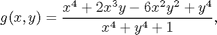
The gradient of a function of several variables is the vector-valued function whose components are the partial derivatives of the function. Let us recall the function f from the previous lesson.
syms x y z
f=((x^2-1)+(y^2-4)+(x^2-1)*(y^2-4))/(x^2+y^2+1)^2
f =

((x^2 - 1)*(y^2 - 4) + x^2 + y^2 - 5)/(x^2 + y^2 + 1)^2
The gradient of f can be computed using the function jacobian from the symbolic toolbox. Notice that a vector whose components are the variables is needed as the second argument to jacobian. It is worth noting that jacobian actually has much more general capabilities, which we will be using later in the course. Incidentally, there is also a MATLAB command called gradient, but it produces a numerical approximation to the gradient, not a symbolic form for the gradient.
gradf=jacobian(f,[x,y])
gradf =

[ (2*x + 2*x*(y^2 - 4))/(x^2 + y^2 + 1)^2 - (4*x*((x^2 - 1)*(y^2 - 4) + x^2 + y^2 - 5))/(x^2 + y^2 + 1)^3, (2*y + 2*y*(x^2 - 1))/(x^2 + y^2 + 1)^2 - (4*y*((x^2 - 1)*(y^2 - 4) + x^2 + y^2 - 5))/(x^2 + y^2 + 1)^3]
We can plot the gradient of f by using quiver. It is particularly interesting to superimpose this on a contour plot of f. Both quiver and contour require using meshgrid first. Note that to get a good picture, you generally need a rather closely spaced mesh for contour, but a sparser one for quiver.
[xx, yy] = meshgrid(-3:.1:3,-3:.1:3);
ffun = @(x,y) eval(vectorize(f));
fxfun = @(x,y) eval(vectorize(gradf(1)));
fyfun = @(x,y) eval(vectorize(gradf(2)));
contour(xx, yy, ffun(xx,yy), 30)
hold on
[xx, yy] = meshgrid(-3:.25:3,-3:.25:3);
quiver(xx, yy, fxfun(xx,yy), fyfun(xx,yy), 0.6)
axis equal tight, hold off
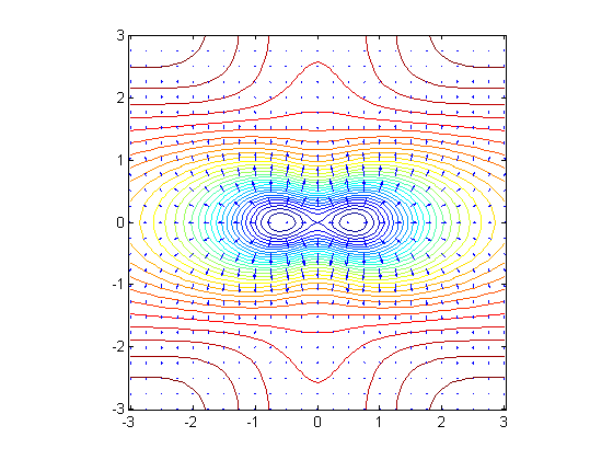
The lengths of the arrows in the gradient plot are determined by both the step size and by the (optional) last numerical parameter to quiver, which we will refer to as the length parameter. What is happening here is that the numerical 'gradient' function is comparing the values of the function at adjacent points on the grid and making the arrows proportional to the difference times the last parameter. It may be necessary to experiment with a few different sets of step sizes and length parameters to get a useful gradient plot. Notice that the gradient arrows are always normal to the level curves. This is always the case.
Behavior Near Critical Points
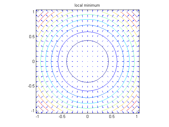
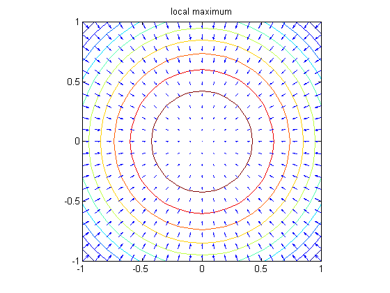
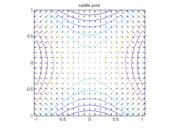
A plot such as this one can be interpreted to give information regarding critical points of the function. Critical points are points where the gradient vector vanishes. A critical point is called on-degenerate if behavior of the function near the critical point is controlled by the second derivatives (so that the 'second derivative test' applies). For functions of two variables, there are three kinds of non-degenerate critical points. You can recognize them from the following three kinds of pictures:
f1 = x^2 + y^2; gradf1 = jacobian(f1,[x,y]);
f1fun = @(x,y) eval(vectorize(f1));
f1xfun = @(x,y) eval(vectorize(gradf1(1)));
f1yfun = @(x,y) eval(vectorize(gradf1(2)));
[xx, yy] = meshgrid(-1:.1:1,-1:.1:1);
contour(xx, yy, f1fun(xx, yy), 10)
hold on
quiver(xx, yy, f1xfun(xx, yy), f1yfun(xx, yy), 0.5)
title('local minimum'), axis equal tight, hold off
set(gca, 'YTick', -1:.5:1)
contour(xx, yy, -f1fun(xx, yy), 10)
hold on
quiver(xx, yy, -f1xfun(xx, yy), -f1yfun(xx, yy), 0.5)
title('local maximum'), axis equal tight, hold off
set(gca, 'YTick', -1:.5:1)
f2 = x^2 - y^2; gradf2 = jacobian(f2,[x,y]);
f2fun = @(x,y) eval(vectorize(f2));
f2xfun = @(x,y) eval(vectorize(gradf2(1)));
f2yfun = @(x,y) eval(vectorize(gradf2(2)));
contour(xx, yy, f2fun(xx, yy), 10)
hold on
quiver(xx, yy, f2xfun(xx, yy), f2yfun(xx, yy), 0.5)
title('saddle point'), axis equal tight, hold off
set(gca, 'YTick', -1:.5:1)
In the case of the function f, we can see that there are two local minima and a saddle point on the x-axis. The two minima can be identified from the fact that they are surrounded by closed contours along which the gradient arrows point outward. The saddle point marks the transition from contours consisting of pairs of closed contours around the two minima, to single curves surrounding both minima. Note that the level curve through a saddle point has a self-intersection. By symmetry, it seems safe to conclude that the saddle point is at the origin, and that the minima are symmetrically placed around it. We will continue to pursue this example in the next notebook.
Problem 1:
- (a) Obtain a simultaneous contour and gradient plot of the function
defined in Problem 1 of the previous lesson.
- (b) Explain what information the plot conveys regarding the location and nature of the critical points of the function.
Gradients of Functions of Three Variables, and Tangent Planes to Surfaces
The three-dimensional analogue of the observation that the gradient of a function of two variables is always normal to the level curves of the function is the fact that the gradient of a three dimensional function is always normal to the level surfaces of the function. It follows that the gradient of the function at any point is normal to the tangent plane at that point to the level surface through that point. This can be exploited to plot the tangent plane to a surface at a chosen point.
Let us plot the surface
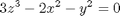
together with its tangent plane at the point (2,4,2). We begin by checking that the indicated point satisfies the equation.
g = 3*z^3-2*x^2-y^2; subs(g,[x,y,z],[2,4,2])
ans =

     0
Next we determine the gradient of g at (2,4,2).
gradg=jacobian(g, [x,y,z])
planenormal=subs(gradg, [x,y,z], [2,4,2])
gradg =

[ (-4)*x, (-2)*y, 9*z^2]


planenormal =

    -8    -8    36
Next we write the function that determines the plane.
realdot = @(u, v) u*transpose(v);
planeq = realdot(planenormal, [x-2,y-4,z-2])
planeq =

36*z - 8*y - 8*x - 24
Then we solve for z in terms of x and y to make this easier to plot.
planefun=solve(planeq,z)
planefun =

(2*x)/9 + (2*y)/9 + 2/3
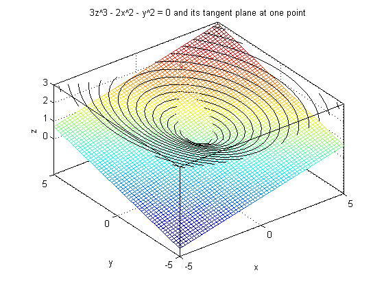
Finally we plot the surface g = 0 and add a plot of the plane so we can see the tangency.
implicitplot3d(g, 0, -5, 5, -5, 5, 0, 3, 20), hold on
plot3(2, 4, 2, 'xr')
ezmesh(planefun, [-5, 5, -5, 5]), hold off
set(gca, 'YTick', -5:5:5, 'ZTick', 0:3)
title '3z^3 - 2x^2 - y^2 = 0 and its tangent plane at one point'
Note that there is another way we could have done this. We could have instead solved for z as a function of x and y in the equation g(x, y, z) = 0 and represented our surface as the graph of a function of two variables: z = h(x, y). Then we could have gotten the equation of the tangent plane from the gradient of h. Here are the details:
h=solve(g,z)
h =

                        (3^(2/3)*(2*x^2 + y^2)^(1/3))/3
  (3^(2/3)*(2*x^2 + y^2)^(1/3)*((3^(1/2)*i)/2 - 1/2))/3
 -(3^(2/3)*(2*x^2 + y^2)^(1/3)*((3^(1/2)*i)/2 + 1/2))/3
Since h should be real, we want the first solution.
h=h(1)
h =

(3^(2/3)*(2*x^2 + y^2)^(1/3))/3
The equation of the tangent plane is then given by:

gradh=simplify(subs(jacobian(h,[x,y]), [x,y], [sym(2),sym(4)]))
planefun=simplify(subs(h,[x,y], [sym(2),sym(4)]))+realdot(gradh,[x-2,y-4])
gradh =

[ 2/9, 2/9]


planefun =

(2*x)/9 + (2*y)/9 + 2/3
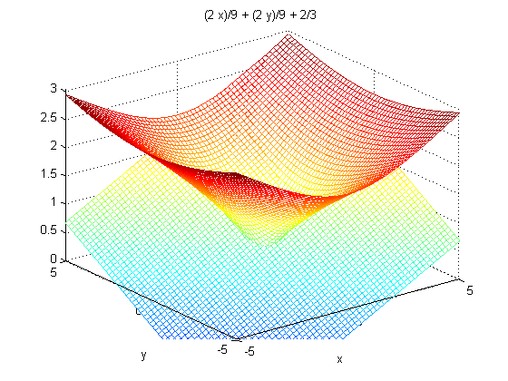
This is the same answer as before. Again we can produce a plot:
ezmesh(h,[-5,5,-5,5]), hold on, ezmesh(planefun,[-5,5,-5,5]), hold off
Problem 2:
Obtain a plot showing the hyperboloid together with its tangent plane at the point (3,4,5).
Additional Problems:
- 1. Obtain simultaneous contour and gradient plots for the function

What information does your plot give you regarding the location and classification of the critical points of in the region -1.5 < x, y < 1.5?
- 2. Obtain a plot showing the ellipsoid
together with its tangent plane at the point (2,3,1).
- 3. Find the equation of the tangent plane to the surface x y z = 8 at the point (-2, -2, 2) in two different ways: by thinking of the surface as a graph of a function of two variables, and also by thinking of the surface as a level surface of a function of three variables. Check that your two answers agree. Then plot the surface (in a vicinity of this point) along with the tangent plane, so that the tangency is visible (you need only do this once).